A radar engineer builds a 5-class object classifier on RadarScenes point clouds. Adding range as a feature improves macro F1 across every validation fold and the final test set. No overfitting in the classical sense. The model just… works better.
But something’s nagging at them. Radar has a physical quirk: the farther an object is, the fewer points it returns. So the model isn’t just learning “this is a car”, it’s learning “far away things are big, big things are vehicles.” Range correlates with object size, and the model might be exploiting that correlation instead of learning actual class distinctions.
This isn’t a theoretical problem. It’s the kind of silent failure that looks great on a benchmark dashboard and falls apart in production.
The Physics Problem Nobody Mentions
Here’s the uncomfortable truth about radar data: it’s sparse, and sparsity is class-correlated. A pedestrian at 20 meters might return 3 points. A truck at 50 meters returns 12. A bicycle at 30 meters might return 1 point, if you’re lucky.
This isn’t random noise. It’s a systematic relationship baked into the sensor physics. Radar cross-section (RCS), detection thresholds, and range all interact to produce point clouds where distance, object size, and point count are hopelessly entangled.
When you train a classifier on this data and feed it range as a feature, you’re giving it a shortcut. The model doesn’t need to learn what distinguishes a pedestrian from a two-wheeler. It can just learn “objects at range X with Y points are probably this class.”
The engineer’s concern is valid: the model may be learning the environment, not the class distribution. And worse, it’s learning that big range means big object.
The Numbers Behind the Concern
The full experiment writeup is public on GitHub, and the findings are sobering.
The baseline model uses a 3-layer MLP with 65-dimension histogram features derived from RCS, compensated velocity, and relative position. The ablation study tested 14 variants, bigger networks, different encodings, alternative binning strategies. Every single variant fell within the split noise floor of 0.651 to 0.734 macro F1.
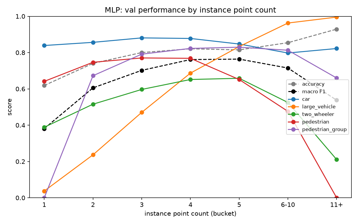
But here’s the kicker: point count alone explains most of the performance ceiling. When the researcher bucketed validation predictions by instance point count, macro F1 jumped from 0.381 at 1 point per instance to 0.764 at 5 points. Same model, same weights, same everything, the only variable was how many radar detections an object happened to produce.
That’s a confound. The model isn’t classifying objects. It’s counting points.
| Point Count | Macro F1 |
|---|---|
| 1 | 0.381 |
| 5 | 0.764 |
The large_vehicle class shows this most dramatically: F1 of 0.037 at 1 point, 0.995 at 11+ points. A single radar detection literally cannot tell you if something is a truck or a car. The model doesn’t know either, it’s just guessing.
Don’t Drop Range Yet
The temptation is to just remove range from the feature vector and accept the performance hit. That’s the wrong move, and here’s why.
The key question isn’t “does range improve F1?” It’s “does range improve F1 because it contains real class information or because it’s acting as a shortcut?”
Range does carry legitimate signal. A pedestrian physically cannot be detected at 200 meters with the same reliability as a truck. If your model needs to distinguish between a distant large vehicle and a nearby pedestrian, range is genuinely informative. Dropping it entirely throws away real information.
The GrowthBook analysis of confounding variables frames this well: the issue isn’t the variable itself, it’s whether the variable is entangled with assignment and outcome in ways that corrupt the causal story.
How to Stress-Test Your Model
If you’re worried your model is learning range instead of objects, here’s the protocol:
1. Slice Your Test Set by Range Bins
This is the cheapest and most revealing test. Take your validation predictions and group them into 10-meter range buckets. Then compute per-class recall within each bucket.
The pattern to watch for: pedestrian recall at 20 meters vs. 70 meters. If it’s 60% at close range and drops to zero at distance while car recall stays flat, your model isn’t classifying pedestrians. It’s deciding “far away = vehicle” and calling it a day.
One practitioner suggested an even more targeted version: train on mostly near/mid-range objects, then test on far-range objects. If performance collapses under distribution shift, range is being used as a shortcut. If it holds up, keeping the feature is justified.
2. Run Permutation Importance on Range
Break the feature. Shuffle range values, recompute F1, and measure the drop. If zeroing out range destroys performance while zeroing out Doppler or RCS barely matters, the model has become a distance classifier wearing an object classifier’s costume.
The full report shows this pattern with compensated velocity, which had a zero-out importance drop of -0.331 while the next highest feature was only -0.080. That’s a model dominated by a single feature, and it raises uncomfortable questions about what happens when that feature’s distribution shifts.
3. Check F1 by Point Count Bucket
This one’s free if you already have predictions. Bucket your validation set by detection count and see how performance scales. If F1 goes from 0.38 to 0.76 as points increase from 1 to 5, the model is struggling with the same sparsity problems, and range might just be a proxy for it.
4. Consider Inverse Propensity Weighting
One approach suggested in the data science community is to make training example importance a function of distance. Near-range objects get downweighted, far-range objects get upweighted, and the model can’t get away with ignoring distant classes.
The F1 Variance Trap
Here’s something the report uncovered that’s sneakier than range confounding: sequence-level correlation inflates apparent split variance.
The research used 6-fold cross-validation with StratifiedGroupKFold, which matches instance count ratios per split. The problem? StratifiedGroupKFold cannot split a sequence. A single tracked object, say, an idling cyclist detected across hundreds of consecutive scans, generates hundreds of correlated instances under one sequence. If that sequence lands in validation, the validation distribution gets skewed by one person’s commute.
The report traced this to two_wheeler, which had a fold-to-fold F1 spread of 0.386. The causal mechanism: vr_compensated (the model’s most important feature, zero-out drop of -0.331) had the largest cross-fold KS statistic for two_wheeler. When the researcher retrained without vr_compensated, the fold-to-fold F1 spread narrowed to 0.133.
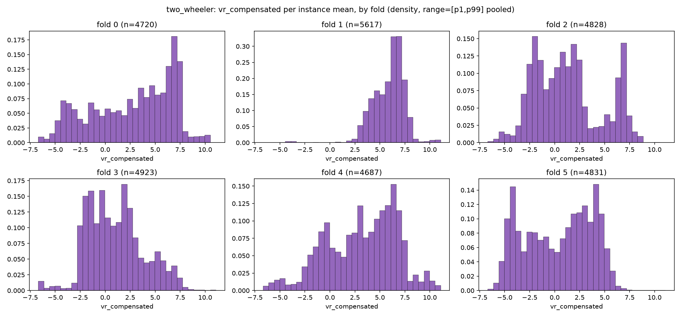
The takeaway is brutal: your model’s F1 score might vary by ±0.04 depending on which specific cyclists happened to be in which data split. That’s not a model problem. That’s a data problem wearing a model problem’s clothing.
Where the Confusion Actually Happens
The confusion matrix tells a story that range bias only partially explains.
Cars vs. large vehicles: Dense point clouds are far more separable (probe AUC of 0.98), yet still show 9.2% real confusion rate. Misclassified cars carry half the decision margin of confident calls and are anomalously wide for their class. The model isn’t confused by range, it’s confused by a wide car with high RCS.
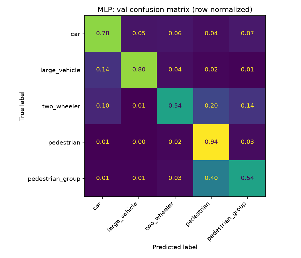
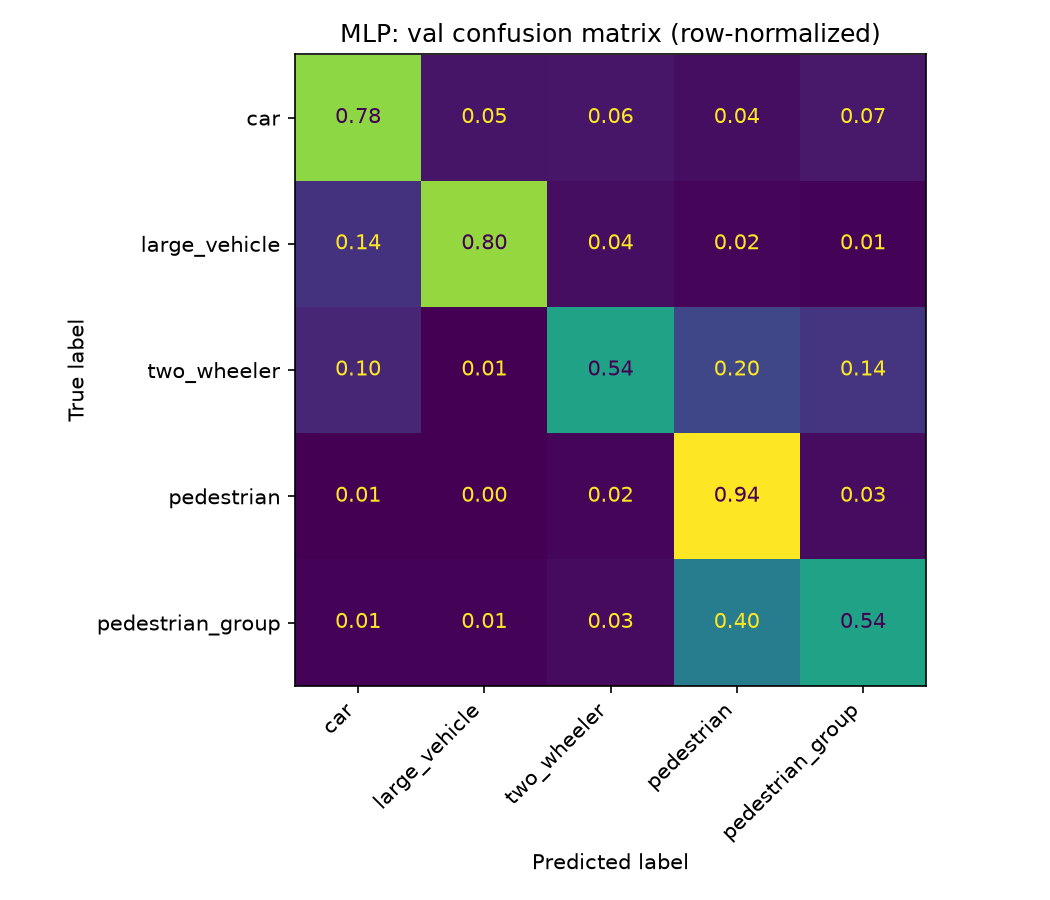
Two-wheelers vs. pedestrians: This is the real mess. Twenty to 24% of two-wheelers get classified as pedestrians, while only 1-2% of pedestrians become two-wheelers. The mechanism: vr_compensated reads near zero for both a stationary pedestrian and an idling cyclist. At that velocity, local instance density favors pedestrians 12:1 in the sparse regime. A true two-wheeler at zero velocity is statistically outvoted.
Even worse: a stationary two-wheeler with a single radar point is physically indistinguishable from a pedestrian. A car with one point gets classified correctly because RCS and Doppler are sufficient for that class. A bike doesn’t have that luxury.
The Taxonomy Problem Nobody Wants to Own
The report highlights a decision that deserves more scrutiny: merging bicycles and motorcycles into a single two_wheeler class. One commenter made a pointed observation: the radar cross-section of a bicycle is nearly zero. The majority of the signal comes from the human riding it.
So a bicycle is, radar-physically, closer to a pedestrian than to a motorcycle. The speeds are more similar, the RCS profiles overlap, and for ADAS purposes, a confused pedestrian-bicycle distinction matters far less than an unidentified motorcycle at 40 mph.
The metrics back this up. two_wheeler has the worst performance of any class, and its velocity distribution instability across splits (0.386 F1 spread) makes any improvement hard to measure. This isn’t just a data scarcity issue, it’s a fundamental category error that’s baked into the dataset.
The Real Fix Isn’t a Better Model
Here’s the conclusion that surprises everyone: two_wheeler doesn’t need a better model. It needs more independent sequences and richer point counts.
The report’s next step is multi-scan accumulation, aggregating a tracked object’s points across multiple scans instead of classifying single-scan instances. This attacks sparsity at the input level rather than the encoding level.
The same logic applies to range confounding. You can’t fix a sensor physics problem with a bigger MLP. You can’t regularize away class-correlated sparsity. You have to fix the data pipeline.
This connects to a broader pattern in applied ML: how LLMs process meaning through vector geometry shows that models learn the statistical structure of their inputs, not some platonic ideal of the task. Feed a model a dataset where distance correlates with size, and it will learn distance. Feed it sparse data where point count predicts class, and it will count points. The model isn’t lazy, it’s optimal. The problem is the data is biased.
Similarly, securing AI agents with sandboxed execution demonstrates that systems need boundaries designed around their failure modes, not their happy paths. Radar classifiers need the same treatment: stress tests that probe for shortcut learning before deployment.
The Verdict
Adding range as a feature isn’t wrong. Dropping it isn’t right. The correct answer requires knowing why range helps, and that requires stress testing.
The protocol is straightforward:
- Slice by range bins and watch for per-class recall collapse at distance
- Run permutation importance on range to see if the model depends on it pathologically
- Check F1 by point count to separate genuine signal from sparsity artifacts
- Test under distribution shift by training on near-range and testing on far-range
- Consider inverse propensity weighting to force the model to pay attention to distant classes
If performance collapses under those tests, range is a shortcut. If it survives, keep the feature and accept the improvement.
But understand this: your model will learn whatever correlates with the labels, whether you intend it to or not. That’s not a bug. That’s what neural networks do.
The question is whether you’re building the real cost of running AI models locally into your deployment plan, or ignoring the hidden costs until production forces you to see them. For radar classification, the hidden cost is a model that works beautifully in validation and fails exactly when it matters: at distance, in sparse conditions, with uncertain classes.
And if you’re designing trust boundaries in edge vs cloud AI inference for autonomous vehicles, remember that shortcut learning isn’t just an accuracy issue. It’s a safety issue. A model that treats “far away” as “big vehicle” doesn’t misclassify data points, it misclassifies the road ahead of a moving car.
The techniques for efficient backend execution for large AI models won’t save you here because the problem isn’t throughput. It’s trustworthiness. You can optimize inference all day and still deploy a model that confidently confuses a cyclist for a pedestrian at 40 meters.
The solution isn’t more compute or clever architectures. It’s acknowledging that radar data has physical constraints, that those constraints create systematic bias, and that your model will happily exploit that bias unless you design experiments to catch it.
Or, as the open-weight models for local AI deployment conversation reminds us: having the most powerful tool means nothing if you don’t understand its failure modes.