Your write latency just spiked from 2ms to 400ms in 90 seconds. No deployment. No traffic spike. CPU at 40%, heap normal, zero GC pressure. You spend two hours optimizing partition keys that didn’t need optimizing. The writes are still slow.
You don’t have an application problem. You have a storage engine problem.
The culprit? Exactly what you didn’t configure: an LSM tree doing what it was designed to do at the worst possible moment.
The Problem with “Write Fast, Read Later”
Every modern database that boasts about write throughput is secretly running an LSM tree underneath. RocksDB. Cassandra. ScyllaDB. TiKV. LevelDB. ClickHouse’s MergeTree. They all made the same bet: optimize for writes, accept the read complexity as the price of admission.
The fundamental insight is brutal in its simplicity. A B-tree writes data in place, finding the right page on disk and modifying it. That’s a random write. The disk head seeks to an arbitrary location, then writes. On spinning disks, that seek takes 5-10ms. On SSDs, it wears out cells unevenly and triggers expensive internal garbage collection.
LSM trees flip the entire model. Instead of writing where the data belongs, they write sequentially. Every write goes to an in-memory buffer, then gets appended to a log file. When the buffer fills up, its contents stream to a new file in one sequential pass. No seeking. No random I/O. Just pure, fast sequential writes.
The dirty secret: This speed is a loan you repay through compaction.
The Write Pipeline: Where Your Data Actually Goes
Every write in an LSM tree starts in the memtable, an in-memory sorted structure, typically a skip list or radix trie. The memtable absorbs writes at memory speed. RocksDB defaults to a 64MB memtable (write_buffer_size), but you can crank it up to 128MB or 256MB on a 32GB machine.
// RocksDB: Tuning the memtable layer
rocksdb::Options options;
options.write_buffer_size = 128 * 1024 * 1024,  // 128MB memtable
options.max_write_buffer_number = 3,             // 3 memtables before stall
options.min_write_buffer_number_to_merge = 1,    // flush after 1 immutable
Before the memtable gets updated, the operation hits the Write-Ahead Log (WAL), an append-only file on disk. This ordering, write ahead, then update memory, is what makes the whole thing durable. If the process crashes mid-write, the WAL replays on restart and the memtable is reconstructed exactly as it was.
The WAL introduces the first form of write amplification: every byte you write gets written to disk twice. Once to the WAL immediately, once to an SSTable when the memtable eventually flushes. That 2x cost buys you durability.
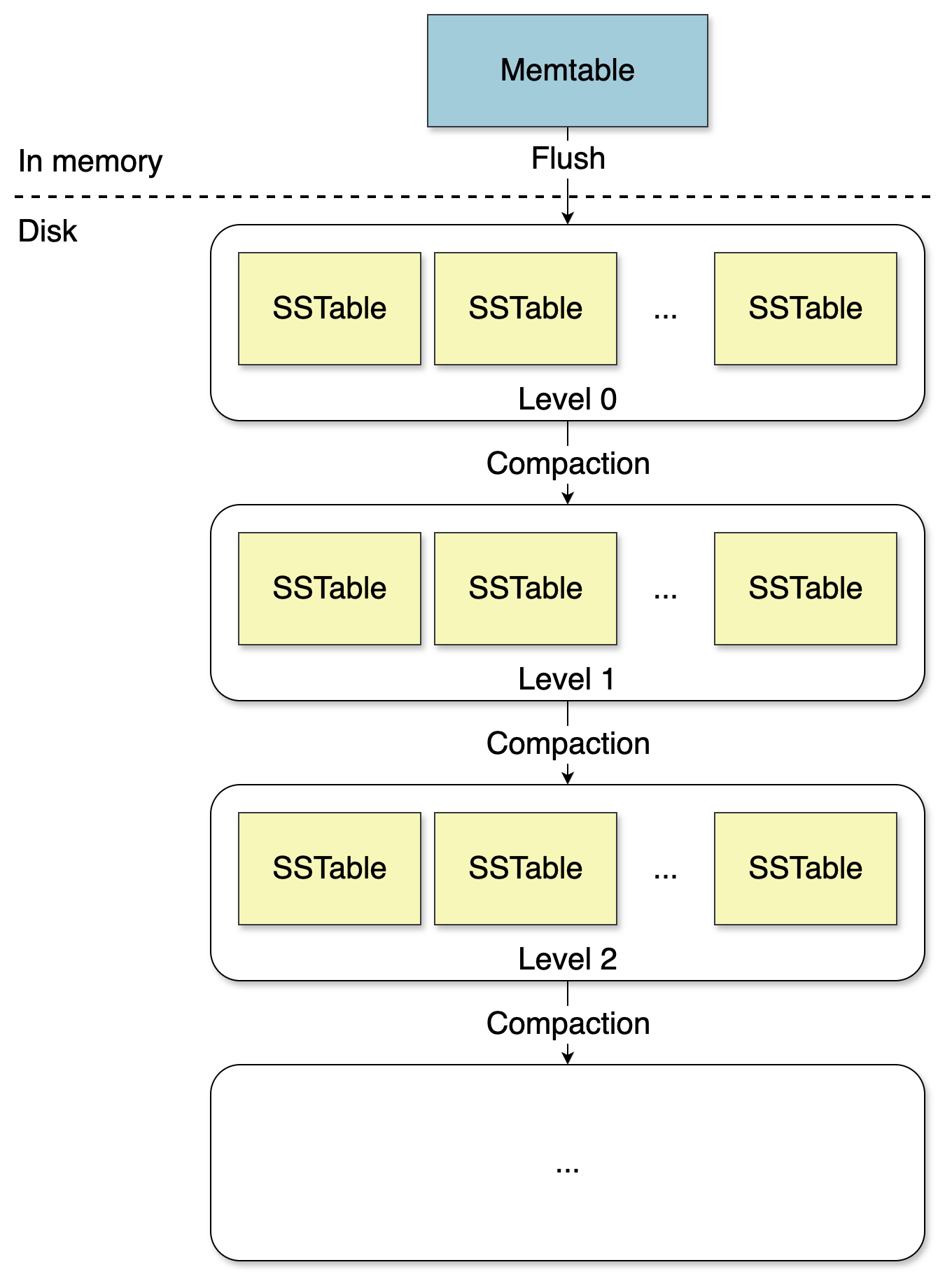
When the memtable fills up, it gets flushed to disk as an SSTable (Sorted String Table), an immutable, sorted file. Immutable means never modified after creation. Sorted means keys are in lexicographic order, making lookups efficient.
A production SSTable isn’t just a flat list. It’s divided into fixed-size blocks (typically 4KB), each with its own checksum. An index block stores the first key of each data block, making binary search possible without reading the entire file. A Bloom filter block lets you skip files entirely for keys that definitely don’t exist.
// RocksDB: Full SSTable configuration
rocksdb::BlockBasedTableOptions table_options;
table_options.filter_policy.reset(rocksdb::NewBloomFilterPolicy(10, false));
table_options.block_size = 4096,  // 4KB blocks
table_options.whole_key_filtering = true;
options.table_factory.reset(rocksdb::NewBlockBasedTableFactory(table_options));
Read Amplification: The Debt Comes Due
This is where the trade-off bites. To look up a key, the engine searches in order of recency: first the active memtable, then immutable memtables waiting to flush, then every SSTable from newest to oldest. The first match wins.
For a key that doesn’t exist, the absolute worst case, the engine must search through every single level before returning “not found.” Each SSTable search is a disk read. This is read amplification: one logical read triggering multiple physical reads.
The RUM conjecture explains this perfectly: a storage engine can excel at two of reads, updates, and memory efficiency, but not all three at once. LSM trees make a deliberate choice: optimize for updates, accept read amplification as the cost.
Bloom filters are what make this survivable. A Bloom filter answers one question with certainty: “Is this key definitely NOT in this SSTable?” No false negatives. If the filter says “not here”, you skip the file entirely, zero I/O. The false positive rate is tunable, at 10 bits per key, you get roughly 1% false positives.
The practical impact is enormous. For a missing key, the engine skips almost every SSTable without a single disk read. Only the rare false positive triggers an unnecessary I/O.
Leveling: Structural Control
Basic compaction, merging all SSTables into one flat pool, doesn’t scale. Enter leveling.
In a leveled LSM tree, SSTables are organized into levels: L0, L1, L2, and so on. Each level has different rules:
- L0 is the landing zone. Files can have overlapping key ranges. When the memtable flushes, the result lands here.
- L1 and deeper maintain non-overlapping key ranges across all files. A given key exists in at most one file per level.
This invariant is critical. To look up a key in L1, you don’t scan all L1 files. You use the key ranges to jump directly to the one file that could contain it.
Each deeper level is typically 10x larger than the previous. L1 might hold 10MB, L2 100MB, L3 1GB. Most data ends up in the deepest level. Most compaction work happens between levels.
The benefit is controlled read amplification: scan all L0 files, then one binary search per deeper level. The number of deeper levels grows logarithmically with data size.

Compaction: The I/O Beast in the Background
Compaction is the background process that merges SSTables, eliminates redundant entries, and reclaims space. It’s also the thing that will wake you up at 3am.
The two strategies that matter are Leveled Compaction and Size-Tiered Compaction, and they trade off differently than the docs suggest:
| Strategy | Write Amp | Read Amp | Space Amp | Best For |
|---|---|---|---|---|
| Leveled | 10-30x | Low | ~1.1x | Read-heavy, mixed |
| Size-Tiered | 3-5x | High | 2-3x | Write-heavy, time-series |
Leveled compaction (RocksDB default) keeps read amplification low at the cost of repeatedly rewriting data as it cascades down levels. Size-tiered compaction (Cassandra default) batches similar-sized SSTables, producing lower write amplification but potentially horrible read performance when many same-level files overlap keys.
// RocksDB: Setting compaction strategy
options.compaction_style = rocksdb::kCompactionStyleLevel,  // or kCompactionStyleUniversal
options.max_bytes_for_level_base = 256 * 1024 * 1024,       // 256MB L1 target
options.level_compaction_dynamic_level_bytes = true,         // let RocksDB scale automatically
The level_compaction_dynamic_level_bytes = true flag is buried in the tuning guide and most tutorials skip it. Without it, you define level sizes statically, and they almost never match actual data growth. With it enabled, RocksDB works backwards from L_max and sizes upper levels proportionally.
The compaction debt problem is what actually bites you in production. Writes land in L0, and compaction is supposed to drain them fast enough that L0 file count stays manageable. RocksDB starts slowing writes at 20 L0 files (level0_slowdown_writes_trigger) and stops writes entirely at 36 (level0_stop_writes_trigger).
If your write rate spikes and compaction threads can’t keep up, L0 fills up and you hit a write stall. The fix requires bumping max_background_compactions from the default to match your core count, and often isolating compaction onto separate NVMe volumes.
On the Cassandra side, nodetool compactionstats is your diagnostic tool:
$ nodetool compactionstats
pending tasks: 847
          id   compaction type   keyspace          table   completed   total    unit    progress
  a1b2c3...   Compaction        my_keyspace       events  102400000   5e9     bytes    2%
A pending tasks number below 50 is healthy. When it climbs past 500, your cluster is accumulating compaction debt faster than it can pay it down.
Deletions: More Expensive Than Writes
Most developers assume deletes are cheap. In an LSM tree, they’re anything but straightforward.
SSTables are immutable. You can’t reach into an existing file and remove an entry. So when a key is deleted, the engine writes a special marker called a tombstone to the memtable. It eventually gets flushed to an SSTable like any other write.
Between when you issue the delete and when compaction finally merges and discards the old data, you have dead records accumulating on disk. Every read has to scan through layers of tombstones before confirming whether a key is alive or dead.
The tricky part is knowing when it’s safe to discard a tombstone during compaction. If a tombstone for key foo exists in a newer SSTable, and an old value for foo exists in an older SSTable that hasn’t been compacted yet, dropping the tombstone without also removing the old value causes data resurrection, deleted data reappears. This is a correctness bug.
The rule: a tombstone can only be dropped when the engine can guarantee that no older value for that key exists anywhere below it on disk.
For time-series data, the fix is to stop issuing explicit deletes entirely and hand the lifecycle off to the storage engine using TTL:
ALTER TABLE events WITH default_time_to_live = 86400;
-- Rows now auto-expire after 24 hours without any application-level delete
TTL-based expiry still writes tombstones internally, but they’re generated predictably and compaction is tuned to handle them efficiently, especially with TimeWindowCompactionStrategy, which groups SSTables by time bucket so tombstones age out in bulk.
Write Amplification: Why Your SSDs Die Young
This is the metric nobody models correctly. Leveled compaction typically delivers 10-30x write amplification. A workload pushing 100MB/s into RocksDB is actually generating 1-3GB/s of real disk I/O behind the scenes.
The math is brutal: a Samsung 980 Pro 2TB has a rated TBW of 1,200TB. At 30x write amplification and 50MB/s apparent write throughput, you’re writing ~1.5GB/s to disk. That entire TBW budget gets blown through in roughly 9 days of continuous operation.
Measuring your actual write amplification is non-negotiable before going to production:
std::string stats;
db->GetProperty("rocksdb.stats", &stats);
// Look for "Cumulative compaction" section
// Write amplification = Cumulative write bytes / bytes flushed from memtable
If you’re seeing above 20x on leveled compaction, your compaction is probably fighting itself. Check whether level_compaction_dynamic_level_bytes is enabled, because without it your L1 size target can drift badly and trigger cascading compactions.
Universal (size-tiered) compaction cuts write amplification to 2-10x, but you pay with space amplification, your on-disk footprint can balloon to 2x the logical data size.
Concurrency and the Versioned Catalog
Everything described so far assumes a single thread. In reality, a storage engine needs to handle concurrent reads and writes while flush and compaction run in the background.
The core problem: a flush operation replaces the current memtable and registers a new SSTable. A compaction operation removes old SSTables and registers new ones. If a read is in the middle of searching an SSTable that gets deleted by concurrent compaction, that’s a crash.
One common solution is a versioned catalog. Every incoming request acquires the latest catalog version, pins it by incrementing a reference count, performs its work, then releases it. Background workers never modify an existing catalog. Instead, when a flush or compaction completes, they create a new catalog version pointing to the updated state.
Old catalog versions are only cleaned up when their reference count drops to zero. No reader is using it anymore, so it’s safe to remove the backed SSTables.
This approach keeps foreground reads and writes lock-free in the hot path. Background operations never block requests, and requests never block background operations. They operate on independent catalog versions and only synchronize at the moment of catalog swap, a single atomic pointer update.
When NOT to Use an LSM-Backed Database
The most common mistake I see teams make is reaching for RocksDB or Cassandra because they read a benchmark showing 500K writes/sec, then spending months debugging why their read latency is 200ms.
Read-heavy workloads with low write rates: If your application is reading 10x more than it writes, a B-Tree store will beat an LSM tree on the same hardware. PostgreSQL’s B-Tree indexes keep data sorted on disk in a way that maps directly to random reads. One I/O, maybe two with a heap fetch. With an LSM tree, a point lookup has to check the memtable, then potentially L0, L1, L2, and deeper levels before finding your key.
The trade-offs between LSM Trees and B-Trees for database storage are well-documented, and the choice is downstream of your access patterns, get that wrong and no amount of tuning saves you.
Random point lookups on cold data: Read amplification is the LSM tree’s original sin. Each level is another potential disk read. If your access pattern is uniformly random across a large keyspace, audit log lookups, sparse sensor data queries, your bloom filters are cold, your block cache is useless, and you’re reading from disk every time.
Short read-modify-write cycles: Counter increments, balance updates, anything that reads a value then writes it back, these are genuinely awkward in LSM-backed stores. Each read in that transaction still pays the read amplification tax, and write-write conflicts under high concurrency cause retry storms that tank throughput.
The Honest B-Tree vs LSM Comparison
On identical hardware, a 3-node cluster of m6i.4xlarge instances, a properly indexed PostgreSQL instance with connection pooling will outperform a Cassandra cluster on mixed OLTP workloads. PostgreSQL can use the full RAM for shared_buffers and OS page cache, index scans are single-digit milliseconds, and you get real transactions without application-level conflict resolution.
Cassandra earns its keep when you need horizontal write scaling beyond what a single Postgres primary can handle, when you genuinely need multi-region active-active writes, or when your data model maps naturally to wide rows.
Performance issues with B-tree-based systems like MySQL under write-heavy loads become obvious at scale, but “we might need to scale later” is not a reason to take on LSM complexity and ops burden today.
For analytics workloads, ClickHouse’s MergeTree engine is the most interesting LSM variant, it writes data in sorted chunks that get merged in the background, but the data is column-oriented within each chunk. You get LSM’s write throughput advantage combined with columnar compression and vectorized reads. The tradeoff: ClickHouse is almost append-only in practice. Updates and deletes rewrite entire parts, which is expensive.
Practical Tuning Checklist
Before you go to production, these are the settings that actually matter:
RocksDB:
1. Set block_cache to 30-50% of available RAM. The default is 8MB, useless for any real workload.
2. Enable full Bloom filters with NewBloomFilterPolicy(10, false). The false argument opts into the improved implementation.
3. Set max_background_jobs to your core count for write-heavy workloads.
4. Enable level_compaction_dynamic_level_bytes = true to avoid cascading compaction problems.
Cassandra:
1. Bump memtable_heap_space on 64GB+ nodes to reduce flush frequency.
2. Monitor nodetool compactionstats, pending tasks should hover near 0.
3. Switch to LeveledCompactionStrategy for read-heavy tables, TimeWindowCompactionStrategy for time-series data.
4. Watch gc_grace_seconds, the default of 10 days accumulates tombstones aggressively on delete-heavy workloads.
Disk layout: Put your WAL and SSTable storage on separate physical disks. The WAL is sequential and loves its own partition. SSTables get random reads during compaction. Mixing them means WAL writes compete with compaction I/O on the same device queue.
# Monitor during load test
iostat -x 1
# util% above 80% sustained = bottleneck
# await above 15ms on NVMe = red flag
You can’t compaction-strategy your way out of a saturated I/O device.
The Bottom Line
LSM trees are a deliberate choice to optimize for writes at the expense of reads. They power the databases that handle millions of writes per second, but they demand understanding the trade-offs. Every tuning decision is a three-way trade-off between write amplification, read amplification, and space amplification. You cannot optimize all three simultaneously.
The challenge of storing and querying JSON data within LSM-based storage engines illustrates exactly this tension, what works beautifully for append-heavy time-series data can fall apart for mixed workloads with complex queries.
The defaults are conservative. They won’t destroy you, but they’re leaving performance on the table for almost every real-world use case. Measure your actual workload. Model your write amplification. Configure your compaction strategy to match your access pattern. Do that, and your LSM-based database will actually deliver on its promises.