
Zero-Shot or Zero Credibility? The Data Leakage Trap in Tabular Foundation Models
Foundation models promise forecasting without training. But the ‘no training’ claim hides a minefield of leakage risks that can sink your backtest.
Electricity prices are among the hardest series to forecast. In Germany, the price for every hour tomorrow is set today in the day-ahead auction. When the wind blows, prices fall and sometimes turn negative. When the wind stops, gas and coal plants set prices that can double from one day to the next.
For this kind of problem, most practitioners reach for LightGBM. It’s the industry default, it’s reliable, and it’s hard to beat. But what if you could skip the training entirely? What if a foundation model that has never seen your data could beat your carefully tuned tree ensemble?
That’s the promise of tabular foundation models (TFMs) like NVIDIA’s Kumo, Synthefy’s Nori, and the TabPFN lineage. And recent benchmarks suggest the hype might be real. But there’s a catch that most discussions gloss over: the “no training” claim is only valid if you can prevent data leakage. And that’s a lot harder than it sounds.
The Workflow That Changes Everything
Here’s the core idea: a TFM is pretrained once across many tables, then applied to a new table by conditioning on its labelled rows, with no training on that table. Think of it like giving examples in a prompt to an LLM, except the “prompt” is a table of historical data.
This is fundamentally different from what we’re used to. A recent regime-stratified critical review published in Electronics asks the question directly: where do TFMs hold a supported advantage over established tabular learners? The answer isn’t “everywhere”, it’s regime-dependent. On small-to-medium independent and identically distributed (IID) tables, TFMs match or exceed tuned tree ensembles without per-dataset tuning. That’s the strong claim.

But here’s the uncomfortable part. The same review found that only 3 of 29 comparison-bearing studies use a deployment-matched split. And 13 of 24 studies evaluating a pretrained model report no contamination or leakage check at all. For a field that’s about to change how enterprises do forecasting, that’s a terrifying gap.
The Leakage Trap Nobody Talks About
When you use a TFM for forecasting, you’re not just loading a model and calling predict(). You’re constructing a table that represents your forecasting problem. And that’s where the leaks creep in.
Let me show you a concrete example from a recent benchmark that pitted Kumo, Nori, Chronos-2, and TimesFM-3 against tuned LightGBM and CatBoost on German day-ahead electricity prices. The setup seems simple: predict tomorrow’s 24 hourly prices using the 30 days of history.
The tabular foundation models need 31 features to capture the problem:
– Calendar features (10): sine and cosine of hour, weekday, month, day of year, weekend and holiday flags
– Fourier terms (14): extra daily, weekly, and yearly waves
– Lags (4): prices from 24, 48, 72, and 168 hours earlier
– Covariates (3): load, renewables, and residual load forecasts
Here’s the trap. If you’re predicting all 24 hours of tomorrow at once, a 1-hour lag for tomorrow at 10:00 is the price at 09:00 tomorrow, which you don’t know yet. A model with that feature looks brilliant in a backtest and utterly fails in production.
The benchmark’s feature code refuses any lag shorter than 24 hours, with a test ensuring no feature reads a price from the block it predicts. That’s not paranoia. That’s the difference between a model that works and one that’s been quietly memorizing your test set.
Why Covariates Are Both a Blessing and a Leak
The most interesting finding from that benchmark isn’t which model won. It’s that covariates decide the result for every model type.
With just the calendar features, Kumo-large scores a MAE of 16.88. Adding Fourier waves brings it to 12.82. Lags change almost nothing. But adding the load, renewables, and residual load forecasts cuts the error to 3.84, more than three times lower. Nori follows the same pattern, from 17.01 down to 4.35.
For electricity, tomorrow’s demand and wind matter far more than recent prices.
But here’s the thing you need to ask yourself: are those covariates truly known at prediction time? The benchmark uses day-ahead forecasts of load and renewables, values published the day before. That’s legitimate. But in many real-world scenarios, what passes for a “known future covariate” is actually a value that gets revised, corrected, or backfilled.
The moment you use a covariate that wasn’t available at decision time, you’ve leaked the future into your context. And your backtest results become worthless.
The One-Day That Decides Everything
Here’s where the benchmark gets genuinely spicy. Over 7 test days, all 4 foundation models beat both tuned trees. Kumo-large had a MAE about 21% lower than LightGBM. Nori about 11% lower. Chronos-2 and TimesFM-3 won by about 3%.
But split the results by day, and the story changes completely. On 5 of the 7 days, the 4 models are within 1 EUR/MWh of each other. Then comes Wednesday, 29 November.
The wind stopped. Wind and solar forecasts fell about 5 times, and residual load jumped. The mean price almost doubled, peaking near 120 EUR/MWh.
Kumo handled it. It searched its 30-day context and found a nearly identical day, 8 November, with almost the same residual load (19,789 MW vs. 19,933 MW) and a similar price spike (120.0 vs. 118.5 EUR/MWh). This is what weather forecasters call the method of analogues: find the most similar past day and check what happened.
Chronos-2 didn’t. Its error was more than twice Kumo’s on that day. The 3 days before 29 November had low prices. Chronos-2 gave a lot of weight to the recent pattern and stayed too low.
Now here’s the kicker: on the 6 “normal” days, Chronos-2 was actually the best model (3.51 vs. 3.64 for Kumo-large). The ranking of the foundation models over the entire week comes from one single day.
This is the risk of short test windows. With 7 forecasts, one day can reorder the models. That’s not a verdict on which model is better, it’s a warning about how fragile your evaluation can be when you’re not careful about your setup.
The Evidence Problem
The Electronics review I mentioned earlier does something rare: it doesn’t just accept TFM claims at face value. It grades 7 recurring claims on a five-dimension rubric: peer review, evaluator independence, split match, baseline strength, and replication.
The findings are sobering.
Only one claim is Strongly supported: TFMs match or exceed tuned tree ensembles on small-to-medium IID tables. The “training-free” claim is contested, supported for accuracy but not for subgroup outcomes until context protocols are disclosed. Claims about predictive distributions, structured-task extensions, and language-model table predictors all remain Preliminary.
And here’s the pattern that should make every practitioner pause: in each of three comparisons where the evaluation broadened, extending the split design from random to temporal, extending the metric from discrimination to conditional coverage, extending the evaluator from developers to independent researchers, the apparent TFM advantage moved towards parity.
A wider evaluation narrows the estimated advantage. Every time.
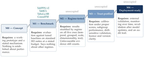
No reviewed model has post-deployment evidence. None reach the top rung of the Evidence Ladder, M4, which requires performance monitored through drift, revalidation after model updates, and an audit trail linking decisions to the artefact that produced them. That’s not a research gap, it’s a deployment gap. And it’s exactly where the data leakage risks live.
When a Tree Is Still the Better Choice
Let me be clear: this isn’t an anti-foundation-model screed. These models are genuinely impressive. But they’re not universal replacements. A tree is still the better choice (for now) when:
- You train once on a very large, stable table and need millions of cheap predictions
- You can’t send a context table at prediction time
Foundation models pay a cost at every forecast because they read the whole context each time. On a MacBook M1, Kumo’s 7 test days took 36 minutes on CPU. A tuned LightGBM predicts almost instantly after training. The trade-off is real.
But for a small, recent, well-prepared table where you want good forecasts with intervals and no training, day-ahead electricity prices are exactly this case, TFMs shine.
The Practical Checklist
Before you run a foundation model on your forecasting problem, ask yourself these questions:
- What does your lag structure reveal? If any feature reads a value from the prediction block, kill it. A 1-hour lag for a 24-hour horizon forecast is leakage.
- Are your covariates genuinely available at decision time? Day-ahead forecasts published yesterday are fine. Revised values or actuals are not.
- What’s your split design? Random splits on temporal data overstate performance. Period.
- Does your context selection use information unavailable in deployment? If you’re selecting context rows based on test labels, your in-context comparison is invalidated.
- Are you checking for contamination? If your model was pretrained on real data, you need provenance checks. Synthetic-prior models have a structural argument for no overlap, but that’s an assumption, not a guarantee.
The TFM Reporting Checklist from the Electronics review consolidates these requirements into a single instrument. Every item exists because at least one study shows that its absence changes the reported result.
The Bottom Line
The “no training” claim of tabular foundation models is technically accurate, and practically misleading. The absence of parameter updates doesn’t mean the absence of choices. Context selection, preprocessing, feature engineering, covariate selection, and split design all become part of the scientific claim. These are the places where data leakage hides.
The data from the electricity benchmark shows something Google’s TabFM also demonstrates: foundation models can beat tuned trees, but their performance depends on getting the setup right. Before you tune a tree for days, run a foundation model zero-shot on the same features. It takes minutes, and it sets the bar your tree has to beat.
Just make sure the bar is measured honestly.
My suggestion: treat the “training-free” claim as a starting point, not a guarantee. TabPFN’s scalability for large tabular datasets makes these models increasingly relevant for production workloads, and Google’s zero-shot foundation model for tabular data is pushing the envelope further. But the risks of using LLMs naively for forecasting apply doubly to foundation models that claim to skip the data engineering entirely.
And if you’re dealing with relational data, the foundation models eliminating the need for manual feature engineering are real, but they still need leakage checks.
The question isn’t whether TFMs can beat LightGBM. It’s whether you’ll know it when they do. One day, and one improperly constructed feature, can change the answer entirely.